Analysis of MTT assay results of EDA-treated astrocytes from multiple experiments
Evgenii O. Tretiakov
2025-06-17
Last updated: 2025-06-17
Checks: 7 0
Knit directory: Cinquina_2024/
This reproducible R Markdown analysis was created with workflowr (version 1.7.1). The Checks tab describes the reproducibility checks that were applied when the results were created. The Past versions tab lists the development history.
Great! Since the R Markdown file has been committed to the Git repository, you know the exact version of the code that produced these results.
Great job! The global environment was empty. Objects defined in the global environment can affect the analysis in your R Markdown file in unknown ways. For reproduciblity it’s best to always run the code in an empty environment.
The command set.seed(20240320) was run prior to running
the code in the R Markdown file. Setting a seed ensures that any results
that rely on randomness, e.g. subsampling or permutations, are
reproducible.
Great job! Recording the operating system, R version, and package versions is critical for reproducibility.
Nice! There were no cached chunks for this analysis, so you can be confident that you successfully produced the results during this run.
Great job! Using relative paths to the files within your workflowr project makes it easier to run your code on other machines.
Great! You are using Git for version control. Tracking code development and connecting the code version to the results is critical for reproducibility.
The results in this page were generated with repository version f653eaf. See the Past versions tab to see a history of the changes made to the R Markdown and HTML files.
Note that you need to be careful to ensure that all relevant files for
the analysis have been committed to Git prior to generating the results
(you can use wflow_publish or
wflow_git_commit). workflowr only checks the R Markdown
file, but you know if there are other scripts or data files that it
depends on. Below is the status of the Git repository when the results
were generated:
Ignored files:
    Ignored:    .Rhistory
    Ignored:    .Rproj.user/
    Ignored:    .pixi/
    Ignored:    data/SCP1290/
    Ignored:    data/azimuth_integrated.rds
Note that any generated files, e.g. HTML, png, CSS, etc., are not included in this status report because it is ok for generated content to have uncommitted changes.
These are the previous versions of the repository in which changes were
made to the R Markdown (analysis/MTT.Rmd) and HTML
(docs/MTT.html) files. If you’ve configured a remote Git
repository (see ?wflow_git_remote), click on the hyperlinks
in the table below to view the files as they were in that past version.
| File | Version | Author | Date | Message |
|---|---|---|---|---|
| Rmd | f653eaf | EugOT | 2025-06-17 | mark correctly neurons and astrocytes |
| Rmd | cccdace | EugOT | 2025-06-17 | rebuild notebook of MTT analysis with more samples |
| html | cccdace | EugOT | 2025-06-17 | rebuild notebook of MTT analysis with more samples |
| Rmd | bd323f5 | EugOT | 2025-06-17 | add separately 1 μM MTT plot |
| html | 9636b47 | Evgenii O. Tretiakov | 2024-07-26 | Build site. |
| Rmd | 373fd42 | Evgenii O. Tretiakov | 2024-07-26 | added MTT analysis figure legends |
| Rmd | 160fe90 | Evgenii O. Tretiakov | 2024-07-26 | added MTT analysis with Glutamate for consistency |
| Rmd | 285dc11 | Evgenii O. Tretiakov | 2024-07-26 | update theme in Rmds |
| html | 1d9d8ea | Evgenii O. Tretiakov | 2024-07-26 | Build site. |
| html | 7a9f863 | Evgenii O. Tretiakov | 2024-07-26 | Build site. |
| html | 5fe5043 | Evgenii O. Tretiakov | 2024-07-26 | fix typos |
| html | 5947ab6 | EugOT | 2024-03-20 | fix typos |
| html | d69bcf7 | EugOT | 2024-03-20 | fix .gitignore |
| Rmd | d09b2f1 | EugOT | 2024-03-20 | calculate cell viability MTT assay |
df <- read_tsv(here(data_dir, "ASTRO_MTT_EPA.tsv"))
df <- df %>%
  tidyr::gather(key = Group, value = Measurement)%>%
  drop_na()

kable(df)| Group | Measurement |
|---|---|
| Ctr_1 | 0.6470000 |
| Ctr_1 | 0.6570000 |
| Ctr_1 | 0.5800000 |
| Ctr_1 | 0.6220000 |
| Ctr_1 | 0.6440000 |
| Ctr_1 | 0.5890000 |
| Ctr_1 | 0.6040000 |
| Ctr_1 | 0.5610000 |
| EPA_5μM_1 | 0.6380000 |
| EPA_5μM_1 | 0.6430000 |
| EPA_5μM_1 | 0.6670000 |
| EPA_5μM_1 | 0.6800000 |
| EPA_5μM_1 | 0.6300000 |
| EPA_5μM_1 | 0.6580000 |
| EPA_5μM_1 | 0.6270000 |
| EPA_5μM_1 | 0.6490000 |
| EPA_10μM_1 | 0.6300000 |
| EPA_10μM_1 | 0.6510000 |
| EPA_10μM_1 | 0.6690000 |
| EPA_10μM_1 | 0.6700000 |
| EPA_10μM_1 | 0.6770000 |
| EPA_10μM_1 | 0.6700000 |
| EPA_10μM_1 | 0.7370000 |
| EPA_10μM_1 | 0.6830000 |
| EPA_30μM_1 | 0.7310000 |
| EPA_30μM_1 | 0.7330000 |
| EPA_30μM_1 | 0.7970000 |
| EPA_30μM_1 | 0.7580000 |
| EPA_30μM_1 | 0.7370000 |
| EPA_30μM_1 | 0.7350000 |
| EPA_30μM_1 | 0.5100000 |
| EPA_30μM_1 | 0.6730000 |
| Ctr_2 | 0.8300000 |
| Ctr_2 | 0.8470000 |
| Ctr_2 | 0.8240000 |
| Ctr_2 | 0.8320000 |
| Ctr_2 | 0.9000000 |
| Ctr_2 | 0.8770000 |
| Ctr_2 | 0.8570000 |
| Ctr_2 | 0.7670000 |
| EPA_5μM_2 | 0.8590000 |
| EPA_5μM_2 | 0.9140000 |
| EPA_5μM_2 | 0.9280000 |
| EPA_5μM_2 | 0.9410000 |
| EPA_5μM_2 | 0.8880000 |
| EPA_5μM_2 | 0.9070000 |
| EPA_5μM_2 | 0.9880000 |
| EPA_5μM_2 | 0.8570000 |
| EPA_10μM_2 | 0.8500000 |
| EPA_10μM_2 | 0.8930000 |
| EPA_10μM_2 | 0.8800000 |
| EPA_10μM_2 | 0.9340000 |
| EPA_10μM_2 | 0.9430000 |
| EPA_10μM_2 | 0.9090000 |
| EPA_10μM_2 | 0.8980000 |
| EPA_10μM_2 | 0.9310000 |
| EPA_30μM_2 | 0.8960000 |
| EPA_30μM_2 | 0.9750000 |
| EPA_30μM_2 | 0.9190000 |
| EPA_30μM_2 | 0.9660000 |
| EPA_30μM_2 | 0.9520000 |
| EPA_30μM_2 | 0.9770000 |
| EPA_30μM_2 | 0.9740000 |
| EPA_30μM_2 | 0.8720000 |
| Ctr_3 | 0.7310000 |
| Ctr_3 | 0.7450000 |
| Ctr_3 | 0.7050000 |
| Ctr_3 | 0.6920000 |
| Ctr_3 | 0.7480000 |
| Ctr_3 | 0.7440000 |
| Ctr_3 | 0.7710000 |
| Ctr_3 | 0.6610000 |
| EPA_5μM_3 | 0.7260000 |
| EPA_5μM_3 | 0.7700000 |
| EPA_5μM_3 | 0.7540000 |
| EPA_5μM_3 | 0.7250000 |
| EPA_5μM_3 | 0.6880000 |
| EPA_5μM_3 | 0.7680000 |
| EPA_5μM_3 | 0.7530000 |
| EPA_5μM_3 | 0.7080000 |
| EPA_10μM_3 | 0.7530000 |
| EPA_10μM_3 | 0.7870000 |
| EPA_10μM_3 | 0.7820000 |
| EPA_10μM_3 | 0.7440000 |
| EPA_10μM_3 | 0.7470000 |
| EPA_10μM_3 | 0.7880000 |
| EPA_10μM_3 | 0.7480000 |
| EPA_10μM_3 | 0.7290000 |
| EPA_30μM_3 | 0.7590000 |
| EPA_30μM_3 | 0.8090000 |
| EPA_30μM_3 | 0.7900000 |
| EPA_30μM_3 | 0.8550000 |
| EPA_30μM_3 | 0.7970000 |
| EPA_30μM_3 | 0.8450000 |
| EPA_30μM_3 | 0.8420000 |
| EPA_30μM_3 | 0.8240000 |
| Ctr_4 | 0.8400000 |
| Ctr_4 | 0.7540000 |
| Ctr_4 | 0.7440000 |
| Ctr_4 | 0.7980000 |
| Ctr_4 | 0.7880000 |
| Ctr_4 | 0.8100000 |
| Ctr_4 | 0.8200000 |
| Ctr_4 | 0.8250000 |
| EPA_5μM_4 | 0.7780000 |
| EPA_5μM_4 | 0.8030000 |
| EPA_5μM_4 | 0.7910000 |
| EPA_5μM_4 | 0.7610000 |
| EPA_5μM_4 | 0.7600000 |
| EPA_5μM_4 | 0.7500000 |
| EPA_5μM_4 | 0.7650000 |
| EPA_5μM_4 | 0.7650000 |
| EPA_10μM_4 | 0.7900000 |
| EPA_10μM_4 | 0.7630000 |
| EPA_10μM_4 | 0.8330000 |
| EPA_10μM_4 | 0.8060000 |
| EPA_10μM_4 | 0.7870000 |
| EPA_10μM_4 | 0.7850000 |
| EPA_10μM_4 | 0.7900000 |
| EPA_10μM_4 | 0.8390000 |
| EPA_30μM_4 | 0.8590000 |
| EPA_30μM_4 | 0.8590000 |
| EPA_30μM_4 | 0.8810000 |
| EPA_30μM_4 | 0.8870000 |
| EPA_30μM_4 | 0.9110000 |
| EPA_30μM_4 | 0.8390000 |
| EPA_30μM_4 | 0.9160000 |
| EPA_30μM_4 | 0.9200000 |
| Ctr_5 | 0.5710000 |
| Ctr_5 | 0.5410000 |
| Ctr_5 | 0.5390000 |
| Ctr_5 | 0.5290000 |
| Ctr_5 | 0.5090000 |
| Ctr_5 | 0.5680000 |
| Ctr_5 | 0.5040000 |
| Ctr_5 | 0.5160000 |
| EPA_5μM_5 | 0.5310000 |
| EPA_5μM_5 | 0.5290000 |
| EPA_5μM_5 | 0.5100000 |
| EPA_5μM_5 | 0.5310000 |
| EPA_5μM_5 | 0.5310000 |
| EPA_5μM_5 | 0.5280000 |
| EPA_5μM_5 | 0.5060000 |
| EPA_5μM_5 | 0.5190000 |
| EPA_10μM_5 | 0.5290000 |
| EPA_10μM_5 | 0.5510000 |
| EPA_10μM_5 | 0.5520000 |
| EPA_10μM_5 | 0.5350000 |
| EPA_10μM_5 | 0.5450000 |
| EPA_10μM_5 | 0.5450000 |
| EPA_10μM_5 | 0.5150000 |
| EPA_10μM_5 | 0.5400000 |
| EPA_30μM_5 | 0.6110000 |
| EPA_30μM_5 | 0.6210000 |
| EPA_30μM_5 | 0.7060000 |
| EPA_30μM_5 | 0.5770000 |
| EPA_30μM_5 | 0.5790000 |
| EPA_30μM_5 | 0.5900000 |
| EPA_30μM_5 | 0.5600000 |
| EPA_30μM_5 | 0.5880000 |
| Ctr_6 | 0.5100000 |
| Ctr_6 | 0.5200000 |
| Ctr_6 | 0.5600000 |
| Ctr_6 | 0.5400000 |
| Ctr_6 | 0.5200000 |
| Ctr_6 | 0.5800000 |
| Ctr_6 | 0.5500000 |
| Ctr_6 | 0.5100000 |
| EPA_5μM_6 | 0.5800000 |
| EPA_5μM_6 | 0.6200000 |
| EPA_5μM_6 | 0.7100000 |
| EPA_5μM_6 | 0.6300000 |
| EPA_5μM_6 | 0.6200000 |
| EPA_5μM_6 | 0.6200000 |
| EPA_5μM_6 | 0.6400000 |
| EPA_5μM_6 | 0.6000000 |
| EPA_10μM_6 | 0.5700000 |
| EPA_10μM_6 | 0.5900000 |
| EPA_10μM_6 | 0.6100000 |
| EPA_10μM_6 | 0.5600000 |
| EPA_10μM_6 | 0.6100000 |
| EPA_10μM_6 | 0.5600000 |
| EPA_10μM_6 | 0.5800000 |
| EPA_10μM_6 | 0.5700000 |
| EPA_30μM_6 | 0.6800000 |
| EPA_30μM_6 | 0.6700000 |
| EPA_30μM_6 | 0.6500000 |
| EPA_30μM_6 | 0.6500000 |
| EPA_30μM_6 | 0.6500000 |
| EPA_30μM_6 | 0.6800000 |
| EPA_30μM_6 | 0.6800000 |
| EPA_30μM_6 | 0.6600000 |
| Ctr_7 | 0.6315370 |
| Ctr_7 | 0.6767187 |
| Ctr_7 | 0.6757631 |
| Ctr_7 | 0.7197545 |
| Ctr_7 | 0.7327356 |
| Ctr_7 | 0.6467031 |
| Ctr_7 | 0.7103541 |
| Ctr_7 | 0.7756199 |
| Ctr_7 | 0.6964314 |
| Ctr_7 | 0.7991241 |
| Ctr_7 | 0.7714853 |
| Ctr_7 | 0.7452136 |
| Ctr_7 | 0.6995220 |
| EPA_1μM_7 | 0.6043768 |
| EPA_1μM_7 | 0.9266503 |
| EPA_1μM_7 | 0.8606042 |
| EPA_1μM_7 | 0.8710704 |
| EPA_1μM_7 | 0.9278893 |
| EPA_1μM_7 | 0.8072892 |
| EPA_1μM_7 | 0.7782893 |
| EPA_1μM_7 | 0.7901075 |
| EPA_5μM_7 | 0.2920579 |
| EPA_5μM_7 | 0.4137877 |
| EPA_5μM_7 | 0.5664762 |
| EPA_5μM_7 | 0.5037649 |
| EPA_5μM_7 | 0.6254405 |
| EPA_5μM_7 | 0.5603325 |
| EPA_5μM_7 | 0.4643089 |
| EPA_5μM_7 | 0.4429826 |
df_glut <- read_tsv(here(data_dir, "ASTRO_MTT_Glut_24h.tsv"), col_types = "d")
df_glut <- df_glut %>%
  tidyr::gather(key = Group, value = Measurement)

kable(df_glut)| Group | Measurement |
|---|---|
| Ctr_1 | 0.702 |
| Ctr_1 | 0.683 |
| Ctr_1 | 0.704 |
| Ctr_1 | 0.714 |
| Ctr_1 | 0.702 |
| Ctr_1 | 0.670 |
| Ctr_1 | 0.688 |
| Ctr_1 | 0.664 |
| Ctr_1 | 0.767 |
| Ctr_1 | 0.723 |
| Ctr_1 | 0.718 |
| Ctr_1 | 0.757 |
| Ctr_1 | 0.710 |
| Ctr_1 | 0.689 |
| Ctr_1 | 0.721 |
| Ctr_1 | 0.674 |
| Glu_1 | 0.703 |
| Glu_1 | 0.740 |
| Glu_1 | 0.715 |
| Glu_1 | 0.825 |
| Glu_1 | 0.715 |
| Glu_1 | 0.755 |
| Glu_1 | 0.710 |
| Glu_1 | 0.685 |
| Glu_1 | 0.679 |
| Glu_1 | 0.746 |
| Glu_1 | 0.729 |
| Glu_1 | 0.693 |
| Glu_1 | 0.748 |
| Glu_1 | 0.723 |
| Glu_1 | 0.700 |
| Glu_1 | 0.744 |
| Ctr_2 | 0.647 |
| Ctr_2 | 0.657 |
| Ctr_2 | 0.580 |
| Ctr_2 | 0.622 |
| Ctr_2 | 0.644 |
| Ctr_2 | 0.589 |
| Ctr_2 | 0.604 |
| Ctr_2 | 0.561 |
| Ctr_2 | 0.590 |
| Ctr_2 | 0.609 |
| Ctr_2 | 0.627 |
| Ctr_2 | 0.613 |
| Ctr_2 | 0.604 |
| Ctr_2 | 0.601 |
| Ctr_2 | 0.586 |
| Ctr_2 | 0.590 |
| Glu_2 | 0.625 |
| Glu_2 | 0.629 |
| Glu_2 | 0.624 |
| Glu_2 | 0.648 |
| Glu_2 | 0.666 |
| Glu_2 | 0.675 |
| Glu_2 | 0.658 |
| Glu_2 | 0.571 |
| Glu_2 | 0.621 |
| Glu_2 | 0.693 |
| Glu_2 | 0.638 |
| Glu_2 | 0.630 |
| Glu_2 | 0.670 |
| Glu_2 | 0.669 |
| Glu_2 | 0.698 |
| Glu_2 | 0.605 |
| Ctr_3 | 0.830 |
| Ctr_3 | 0.847 |
| Ctr_3 | 0.824 |
| Ctr_3 | 0.832 |
| Ctr_3 | 0.900 |
| Ctr_3 | 0.877 |
| Ctr_3 | 0.857 |
| Ctr_3 | 0.767 |
| Ctr_3 | 0.803 |
| Ctr_3 | 0.855 |
| Ctr_3 | 0.823 |
| Ctr_3 | 0.818 |
| Ctr_3 | 0.783 |
| Ctr_3 | 0.799 |
| Ctr_3 | 0.833 |
| Ctr_3 | 0.855 |
| Glu_3 | 0.844 |
| Glu_3 | 0.961 |
| Glu_3 | 0.910 |
| Glu_3 | 0.965 |
| Glu_3 | 0.939 |
| Glu_3 | 0.891 |
| Glu_3 | 0.908 |
| Glu_3 | 0.855 |
| Glu_3 | 0.915 |
| Glu_3 | 0.927 |
| Glu_3 | 0.943 |
| Glu_3 | 0.913 |
| Glu_3 | 0.969 |
| Glu_3 | 0.947 |
| Glu_3 | 0.875 |
| Glu_3 | 0.826 |
| Ctr_4 | 0.731 |
| Ctr_4 | 0.745 |
| Ctr_4 | 0.705 |
| Ctr_4 | 0.692 |
| Ctr_4 | 0.748 |
| Ctr_4 | 0.744 |
| Ctr_4 | 0.771 |
| Ctr_4 | 0.661 |
| Ctr_4 | 0.698 |
| Ctr_4 | 0.691 |
| Ctr_4 | 0.682 |
| Ctr_4 | 0.668 |
| Ctr_4 | 0.672 |
| Ctr_4 | 0.715 |
| Ctr_4 | 0.707 |
| Ctr_4 | 0.659 |
| Glu_4 | 0.713 |
| Glu_4 | 0.734 |
| Glu_4 | 0.729 |
| Glu_4 | 0.736 |
| Glu_4 | 0.678 |
| Glu_4 | 0.718 |
| Glu_4 | 0.735 |
| Glu_4 | 0.662 |
| Glu_4 | 0.724 |
| Glu_4 | 0.711 |
| Glu_4 | 0.703 |
| Glu_4 | 0.716 |
| Glu_4 | 0.673 |
| Glu_4 | 0.711 |
| Glu_4 | 0.704 |
| Glu_4 | 0.659 |
| Ctr_5 | 0.840 |
| Ctr_5 | 0.754 |
| Ctr_5 | 0.744 |
| Ctr_5 | 0.798 |
| Ctr_5 | 0.788 |
| Ctr_5 | 0.810 |
| Ctr_5 | 0.820 |
| Ctr_5 | 0.825 |
| Ctr_5 | 0.818 |
| Ctr_5 | 0.773 |
| Ctr_5 | 0.759 |
| Ctr_5 | 0.760 |
| Ctr_5 | 0.741 |
| Ctr_5 | 0.755 |
| Ctr_5 | 0.744 |
| Ctr_5 | 0.737 |
| Glu_5 | 0.784 |
| Glu_5 | 0.757 |
| Glu_5 | 0.779 |
| Glu_5 | 0.789 |
| Glu_5 | 0.757 |
| Glu_5 | 0.784 |
| Glu_5 | 0.751 |
| Glu_5 | 0.795 |
| Glu_5 | 0.777 |
| Glu_5 | 0.726 |
| Glu_5 | 0.718 |
| Glu_5 | 0.739 |
| Glu_5 | 0.762 |
| Glu_5 | 0.737 |
| Glu_5 | 0.776 |
| Glu_5 | 0.778 |
| Ctr_6 | 0.571 |
| Ctr_6 | 0.541 |
| Ctr_6 | 0.539 |
| Ctr_6 | 0.529 |
| Ctr_6 | 0.509 |
| Ctr_6 | 0.568 |
| Ctr_6 | 0.504 |
| Ctr_6 | 0.516 |
| Ctr_6 | 0.494 |
| Ctr_6 | 0.491 |
| Ctr_6 | 0.491 |
| Ctr_6 | 0.486 |
| Ctr_6 | 0.504 |
| Ctr_6 | 0.513 |
| Ctr_6 | 0.521 |
| Ctr_6 | 0.504 |
| Glu_6 | 0.543 |
| Glu_6 | 0.536 |
| Glu_6 | 0.540 |
| Glu_6 | 0.572 |
| Glu_6 | 0.518 |
| Glu_6 | 0.534 |
| Glu_6 | 0.526 |
| Glu_6 | 0.523 |
| Glu_6 | 0.514 |
| Glu_6 | 0.516 |
| Glu_6 | 0.514 |
| Glu_6 | 0.505 |
| Glu_6 | 0.503 |
| Glu_6 | 0.504 |
| Glu_6 | 0.529 |
| Glu_6 | 0.503 |
1 and 5 μM of EPA on Neurons - Figure S7a
unpaired1 <- load(df,
  x = Group, y = Measurement,
  idx = list(
    c("Ctr_7", "EPA_1μM_7", "EPA_5μM_7")
  )
)print(unpaired1)DABESTR v2025.3.14
==================
Good afternoon!
The current time is 16:40 PM on Tuesday June 17, 2025.
ffect size(s) with 95% confidence intervals will be computed for:
1. EPA_1μM_7 minus Ctr_7
2. EPA_5μM_7 minus Ctr_7
5000 resamples will be used to generate the effect size bootstraps.unpaired1.mean_diff <- mean_diff(unpaired1)
print(unpaired1.mean_diff)DABESTR v2025.3.14
==================
Good afternoon!
The current time is 16:40 PM on Tuesday June 17, 2025.
The character(0) mean difference between EPA_1μM_7 and Ctr_7 is 0.107 [95%CI 0.015, 0.168].
The p-value of the two-sided permutation t-test is 0.0242, calculated for legacy purposes only.
The character(0) mean difference between EPA_5μM_7 and Ctr_7 is -0.23 [95%CI -0.309, -0.162].
The p-value of the two-sided permutation t-test is 0.0003, calculated for legacy purposes only.
5000 bootstrap samples were taken; the confidence interval is bias-corrected and accelerated.
Any p-value reported is the probability of observing the effect size (or greater),
assuming the null hypothesis of zero difference is true.
For each p-value, 5000 reshuffles of the control and test labels were performed.kable(unpaired1.mean_diff$boot_result |> select(-bootstraps))| control_group | test_group | nboots | bca_ci_low | bca_ci_high | pct_ci_low | pct_ci_high | ci | difference | weight |
|---|---|---|---|---|---|---|---|---|---|
| Ctr_7 | EPA_1μM_7 | 5000 | 0.0153402 | 0.1678771 | 0.0277831 | 0.1742437 | 95 | 0.1068644 | 177.6146 |
| Ctr_7 | EPA_5μM_7 | 5000 | -0.3091020 | -0.1622632 | -0.3050414 | -0.1592285 | 95 | -0.2302763 | 177.0996 |
dabest_plot(unpaired1.mean_diff)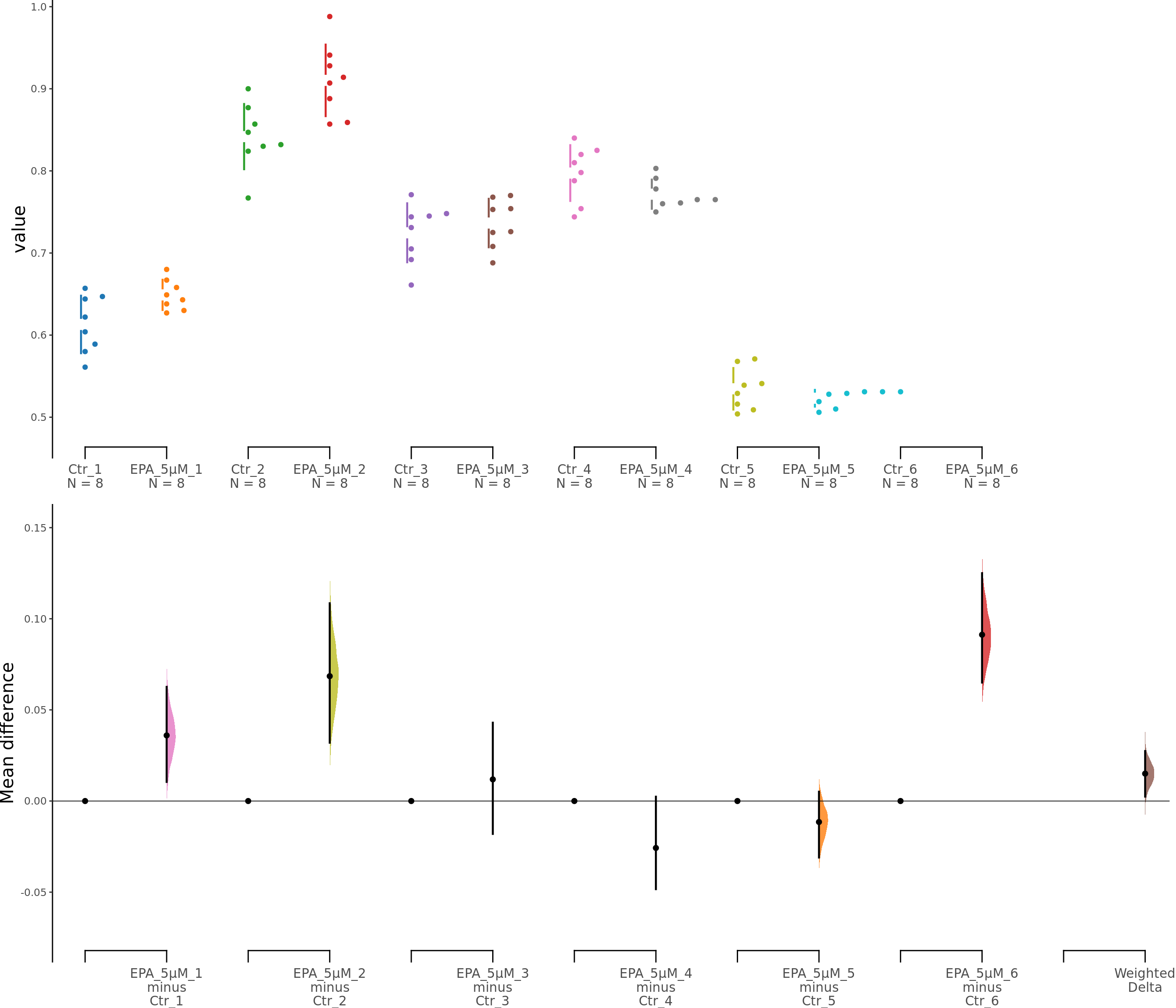
5 μM of EPA on Astrocytes - Figure S7c1
unpaired5 <- load(df,
  x = Group, y = Measurement,
  idx = list(
    c("Ctr_1", "EPA_5μM_1"),
    c("Ctr_2", "EPA_5μM_2"),
    c("Ctr_3", "EPA_5μM_3"),
    c("Ctr_4", "EPA_5μM_4"),
    c("Ctr_5", "EPA_5μM_5"),
    c("Ctr_6", "EPA_5μM_6")
  ),
  minimeta = TRUE
)print(unpaired5)DABESTR v2025.3.14
==================
Good afternoon!
The current time is 16:40 PM on Tuesday June 17, 2025.
ffect size(s) with 95% confidence intervals will be computed for:
1. EPA_5μM_1 minus Ctr_1
2. EPA_5μM_2 minus Ctr_2
3. EPA_5μM_3 minus Ctr_3
4. EPA_5μM_4 minus Ctr_4
5. EPA_5μM_5 minus Ctr_5
6. EPA_5μM_6 minus Ctr_6
7. weighted delta (only for mean difference)
5000 resamples will be used to generate the effect size bootstraps.unpaired5.mean_diff <- mean_diff(unpaired5)
print(unpaired5.mean_diff)DABESTR v2025.3.14
==================
Good afternoon!
The current time is 16:40 PM on Tuesday June 17, 2025.
The character(0) mean difference between EPA_5μM_1 and Ctr_1 is 0.036 [95%CI 0.011, 0.063].
The p-value of the two-sided permutation t-test is 0.0266, calculated for legacy purposes only.
The character(0) mean difference between EPA_5μM_2 and Ctr_2 is 0.068 [95%CI 0.032, 0.109].
The p-value of the two-sided permutation t-test is 0.0055, calculated for legacy purposes only.
The character(0) mean difference between EPA_5μM_3 and Ctr_3 is 0.012 [95%CI -0.018, 0.043].
The p-value of the two-sided permutation t-test is 0.4823, calculated for legacy purposes only.
The character(0) mean difference between EPA_5μM_4 and Ctr_4 is -0.026 [95%CI -0.048, 0.002].
The p-value of the two-sided permutation t-test is 0.0849, calculated for legacy purposes only.
The character(0) mean difference between EPA_5μM_5 and Ctr_5 is -0.011 [95%CI -0.031, 0.005].
The p-value of the two-sided permutation t-test is 0.2624, calculated for legacy purposes only.
The character(0) mean difference between EPA_5μM_6 and Ctr_6 is 0.091 [95%CI 0.065, 0.125].
The p-value of the two-sided permutation t-test is 0.0001, calculated for legacy purposes only.
5000 bootstrap samples were taken; the confidence interval is bias-corrected and accelerated.
Any p-value reported is the probability of observing the effect size (or greater),
assuming the null hypothesis of zero difference is true.
For each p-value, 5000 reshuffles of the control and test labels were performed.kable(unpaired5.mean_diff$boot_result |> select(-bootstraps))| control_group | test_group | nboots | bca_ci_low | bca_ci_high | pct_ci_low | pct_ci_high | ci | difference | weight |
|---|---|---|---|---|---|---|---|---|---|
| Ctr_1 | EPA_5μM_1 | 5000 | 0.0105000 | 0.0626250 | 0.0105000 | 0.0625000 | 95 | 0.036000 | 1278.3053 |
| Ctr_2 | EPA_5μM_2 | 5000 | 0.0320000 | 0.1085000 | 0.0315031 | 0.1076250 | 95 | 0.068500 | 575.6816 |
| Ctr_3 | EPA_5μM_3 | 5000 | -0.0180310 | 0.0429689 | -0.0182469 | 0.0428750 | 95 | 0.011875 | 925.5663 |
| Ctr_4 | EPA_5μM_4 | 5000 | -0.0483460 | 0.0023750 | -0.0494969 | 0.0003719 | 95 | -0.025750 | 1362.6962 |
| Ctr_5 | EPA_5μM_5 | 5000 | -0.0310000 | 0.0051207 | -0.0300000 | 0.0057500 | 95 | -0.011500 | 2693.9914 |
| Ctr_6 | EPA_5μM_6 | 5000 | 0.0650000 | 0.1250000 | 0.0625000 | 0.1225000 | 95 | 0.091250 | 949.9576 |
| Minimeta Overall Test | Minimeta Overall Test | 5000 | 0.0024303 | 0.0274285 | 0.0148743 | 0.0152279 | 95 | 0.015034 | 1.0000 |
dabest_plot(unpaired5.mean_diff)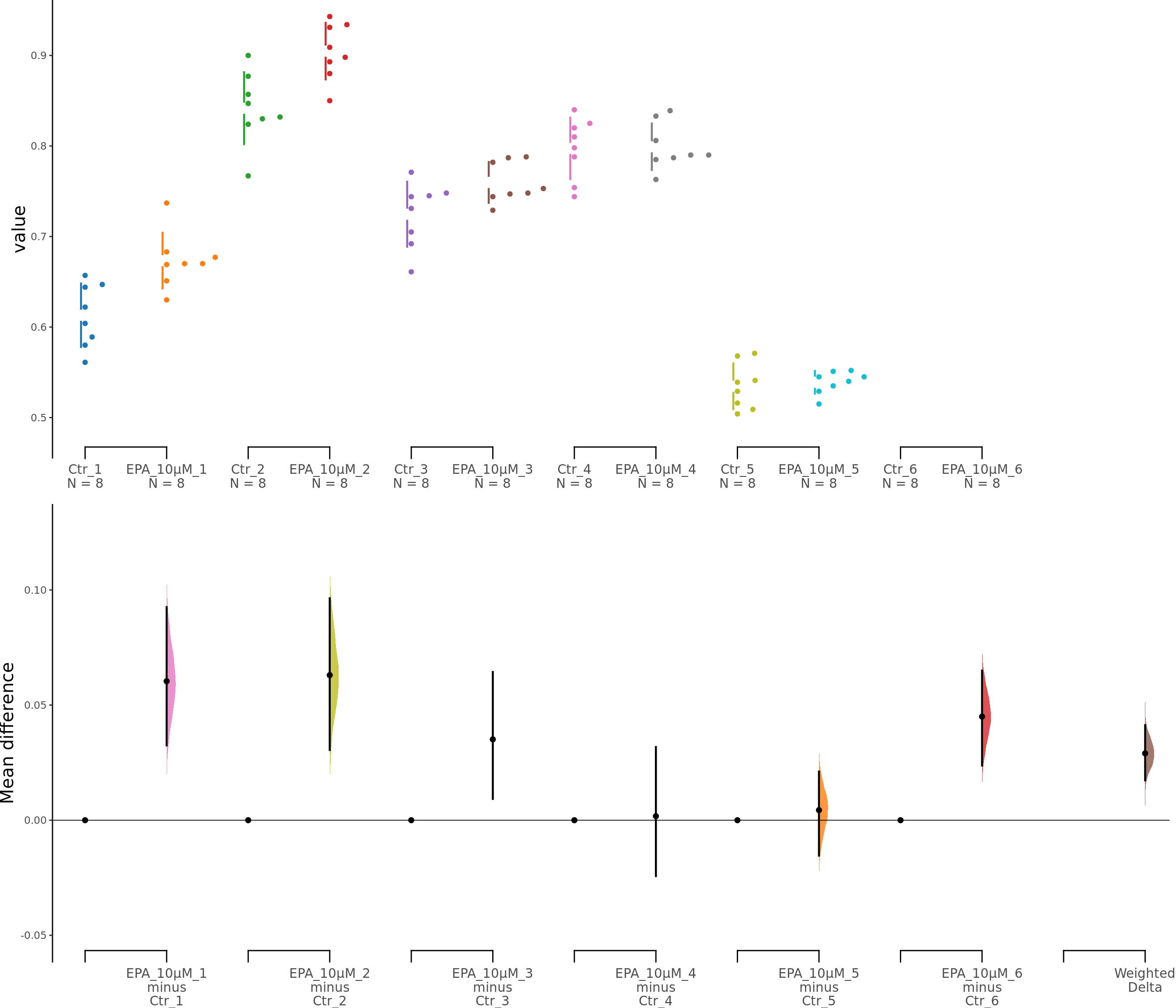
10 μM of EPA on Astrocytes - Figure S7c2
unpaired10 <- load(df,
  x = Group, y = Measurement,
  idx = list(
    c("Ctr_1", "EPA_10μM_1"),
    c("Ctr_2", "EPA_10μM_2"),
    c("Ctr_3", "EPA_10μM_3"),
    c("Ctr_4", "EPA_10μM_4"),
    c("Ctr_5", "EPA_10μM_5"),
    c("Ctr_6", "EPA_10μM_6")
  ),
  minimeta = TRUE
)print(unpaired10)DABESTR v2025.3.14
==================
Good afternoon!
The current time is 16:40 PM on Tuesday June 17, 2025.
ffect size(s) with 95% confidence intervals will be computed for:
1. EPA_10μM_1 minus Ctr_1
2. EPA_10μM_2 minus Ctr_2
3. EPA_10μM_3 minus Ctr_3
4. EPA_10μM_4 minus Ctr_4
5. EPA_10μM_5 minus Ctr_5
6. EPA_10μM_6 minus Ctr_6
7. weighted delta (only for mean difference)
5000 resamples will be used to generate the effect size bootstraps.unpaired10.mean_diff <- mean_diff(unpaired10)
print(unpaired10.mean_diff)DABESTR v2025.3.14
==================
Good afternoon!
The current time is 16:40 PM on Tuesday June 17, 2025.
The character(0) mean difference between EPA_10μM_1 and Ctr_1 is 0.06 [95%CI 0.033, 0.093].
The p-value of the two-sided permutation t-test is 0.0026, calculated for legacy purposes only.
The character(0) mean difference between EPA_10μM_2 and Ctr_2 is 0.063 [95%CI 0.03, 0.096].
The p-value of the two-sided permutation t-test is 0.0036, calculated for legacy purposes only.
The character(0) mean difference between EPA_10μM_3 and Ctr_3 is 0.035 [95%CI 0.009, 0.064].
The p-value of the two-sided permutation t-test is 0.0376, calculated for legacy purposes only.
The character(0) mean difference between EPA_10μM_4 and Ctr_4 is 0.002 [95%CI -0.024, 0.032].
The p-value of the two-sided permutation t-test is 0.9092, calculated for legacy purposes only.
The character(0) mean difference between EPA_10μM_5 and Ctr_5 is 0.004 [95%CI -0.015, 0.021].
The p-value of the two-sided permutation t-test is 0.6694, calculated for legacy purposes only.
The character(0) mean difference between EPA_10μM_6 and Ctr_6 is 0.045 [95%CI 0.024, 0.065].
The p-value of the two-sided permutation t-test is 0.0018, calculated for legacy purposes only.
5000 bootstrap samples were taken; the confidence interval is bias-corrected and accelerated.
Any p-value reported is the probability of observing the effect size (or greater),
assuming the null hypothesis of zero difference is true.
For each p-value, 5000 reshuffles of the control and test labels were performed.kable(unpaired10.mean_diff$boot_result |> select(-bootstraps))| control_group | test_group | nboots | bca_ci_low | bca_ci_high | pct_ci_low | pct_ci_high | ci | difference | weight |
|---|---|---|---|---|---|---|---|---|---|
| Ctr_1 | EPA_10μM_1 | 5000 | 0.0325000 | 0.0925793 | 0.0316250 | 0.0911250 | 95 | 0.0603750 | 923.3686 |
| Ctr_2 | EPA_10μM_2 | 5000 | 0.0305000 | 0.0963750 | 0.0300031 | 0.0960000 | 95 | 0.0630000 | 784.2698 |
| Ctr_3 | EPA_10μM_3 | 5000 | 0.0092500 | 0.0643750 | 0.0083750 | 0.0631250 | 95 | 0.0351250 | 1110.9899 |
| Ctr_4 | EPA_10μM_4 | 5000 | -0.0242500 | 0.0317707 | -0.0257500 | 0.0306250 | 95 | 0.0017500 | 1104.7326 |
| Ctr_5 | EPA_10μM_5 | 5000 | -0.0153750 | 0.0211250 | -0.0143750 | 0.0220000 | 95 | 0.0043750 | 2523.4887 |
| Ctr_6 | EPA_10μM_6 | 5000 | 0.0237500 | 0.0650000 | 0.0237500 | 0.0650000 | 95 | 0.0450000 | 1872.9097 |
| Minimeta Overall Test | Minimeta Overall Test | 5000 | 0.0172908 | 0.0412704 | 0.0289180 | 0.0292622 | 95 | 0.0290195 | 1.0000 |
dabest_plot(unpaired10.mean_diff)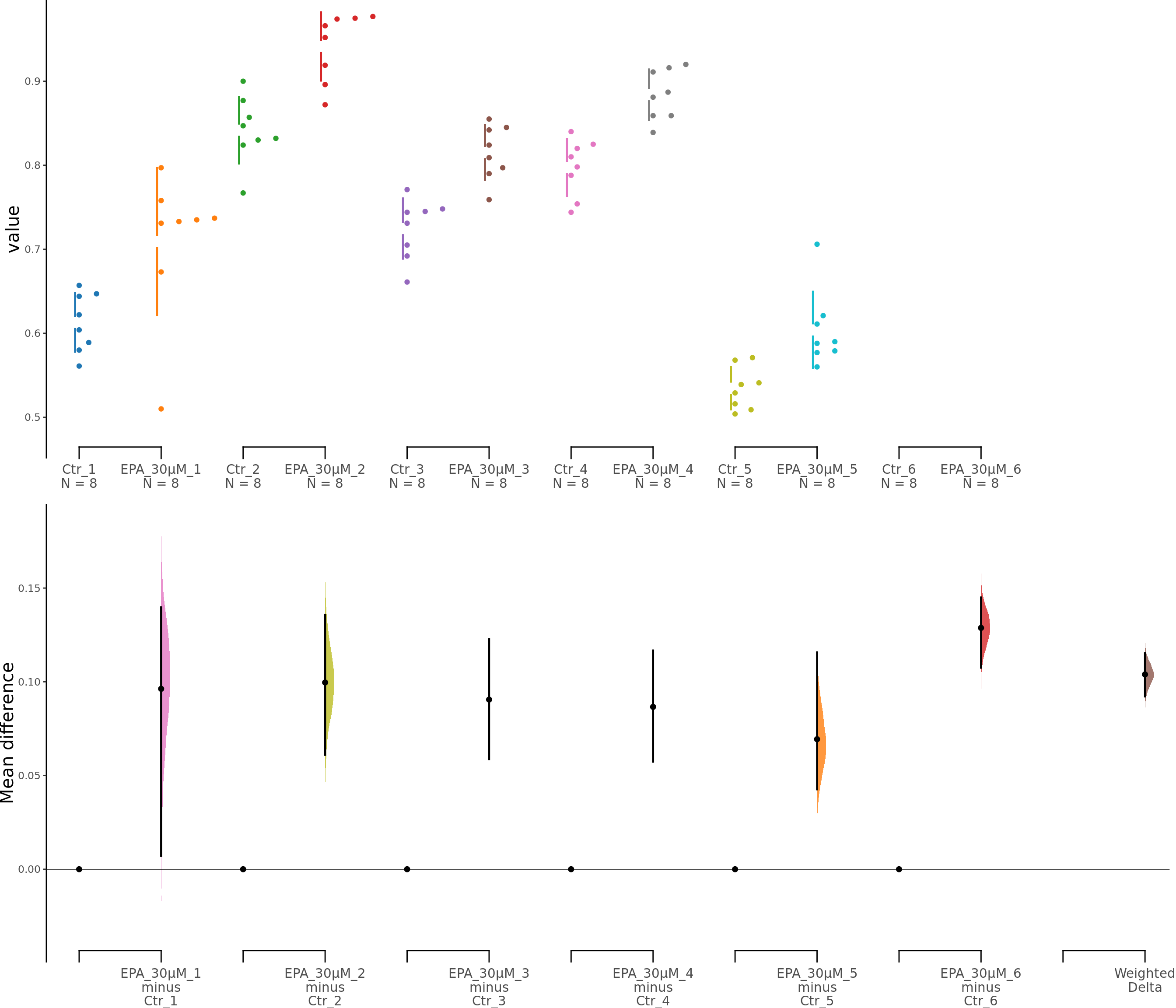
Supplementary Figure 5. Effects of low EPA concentrations on astrocyte viability. b, b1. Cumming estimation plots showing astroglia viability (MTT assay) after 5 μM (b) or 10 μM (b1) EPA treatment. Left panel: Colored circles represent individual data points for control (Ctr) and EPA-treated groups from 6 independent experiments. Black circles and vertical lines indicate group means with 95% confidence intervals. Right panel: Floating plots show mean differences (EPA minus Ctr) for each experiment and the overall weighted mean difference (bottom). Circles represent the point estimate of the mean difference, with vertical lines indicating 95% confidence intervals. The shaded curve represents the resampled distribution of the effect size.
30 μM of EPA on Astrocytes - Figure S7c3
unpaired30 <- load(df,
  x = Group, y = Measurement,
  idx = list(
    c("Ctr_1", "EPA_30μM_1"),
    c("Ctr_2", "EPA_30μM_2"),
    c("Ctr_3", "EPA_30μM_3"),
    c("Ctr_4", "EPA_30μM_4"),
    c("Ctr_5", "EPA_30μM_5"),
    c("Ctr_6", "EPA_30μM_6")
  ),
  minimeta = TRUE
)print(unpaired30)DABESTR v2025.3.14
==================
Good afternoon!
The current time is 16:40 PM on Tuesday June 17, 2025.
ffect size(s) with 95% confidence intervals will be computed for:
1. EPA_30μM_1 minus Ctr_1
2. EPA_30μM_2 minus Ctr_2
3. EPA_30μM_3 minus Ctr_3
4. EPA_30μM_4 minus Ctr_4
5. EPA_30μM_5 minus Ctr_5
6. EPA_30μM_6 minus Ctr_6
7. weighted delta (only for mean difference)
5000 resamples will be used to generate the effect size bootstraps.unpaired30.mean_diff <- mean_diff(unpaired30)
print(unpaired30.mean_diff)DABESTR v2025.3.14
==================
Good afternoon!
The current time is 16:40 PM on Tuesday June 17, 2025.
The character(0) mean difference between EPA_30μM_1 and Ctr_1 is 0.096 [95%CI 0.007, 0.14].
The p-value of the two-sided permutation t-test is 0.0175, calculated for legacy purposes only.
The character(0) mean difference between EPA_30μM_2 and Ctr_2 is 0.1 [95%CI 0.061, 0.136].
The p-value of the two-sided permutation t-test is 0.0002, calculated for legacy purposes only.
The character(0) mean difference between EPA_30μM_3 and Ctr_3 is 0.091 [95%CI 0.059, 0.123].
The p-value of the two-sided permutation t-test is 0.0001, calculated for legacy purposes only.
The character(0) mean difference between EPA_30μM_4 and Ctr_4 is 0.087 [95%CI 0.057, 0.117].
The p-value of the two-sided permutation t-test is 0.0001, calculated for legacy purposes only.
The character(0) mean difference between EPA_30μM_5 and Ctr_5 is 0.069 [95%CI 0.043, 0.116].
The p-value of the two-sided permutation t-test is 0.0031, calculated for legacy purposes only.
The character(0) mean difference between EPA_30μM_6 and Ctr_6 is 0.129 [95%CI 0.108, 0.145].
The p-value of the two-sided permutation t-test is 0.0000, calculated for legacy purposes only.
5000 bootstrap samples were taken; the confidence interval is bias-corrected and accelerated.
Any p-value reported is the probability of observing the effect size (or greater),
assuming the null hypothesis of zero difference is true.
For each p-value, 5000 reshuffles of the control and test labels were performed.kable(unpaired30.mean_diff$boot_result |> select(-bootstraps))| control_group | test_group | nboots | bca_ci_low | bca_ci_high | pct_ci_low | pct_ci_high | ci | difference | weight |
|---|---|---|---|---|---|---|---|---|---|
| Ctr_1 | EPA_30μM_1 | 5000 | 0.0070740 | 0.1397500 | 0.0288781 | 0.1503750 | 95 | 0.0962500 | 225.2778 |
| Ctr_2 | EPA_30μM_2 | 5000 | 0.0610000 | 0.1357500 | 0.0618813 | 0.1367500 | 95 | 0.0996250 | 619.8153 |
| Ctr_3 | EPA_30μM_3 | 5000 | 0.0587500 | 0.1227395 | 0.0585031 | 0.1224969 | 95 | 0.0905000 | 850.7148 |
| Ctr_4 | EPA_30μM_4 | 5000 | 0.0573750 | 0.1167127 | 0.0570000 | 0.1165000 | 95 | 0.0866250 | 971.4211 |
| Ctr_5 | EPA_30μM_5 | 5000 | 0.0426250 | 0.1157298 | 0.0385000 | 0.1073750 | 95 | 0.0693750 | 738.6352 |
| Ctr_6 | EPA_30μM_6 | 5000 | 0.1075000 | 0.1450000 | 0.1087500 | 0.1462500 | 95 | 0.1287500 | 2338.2046 |
| Minimeta Overall Test | Minimeta Overall Test | 5000 | 0.0921689 | 0.1152220 | 0.1037444 | 0.1040722 | 95 | 0.1039085 | 1.0000 |
dabest_plot(unpaired30.mean_diff)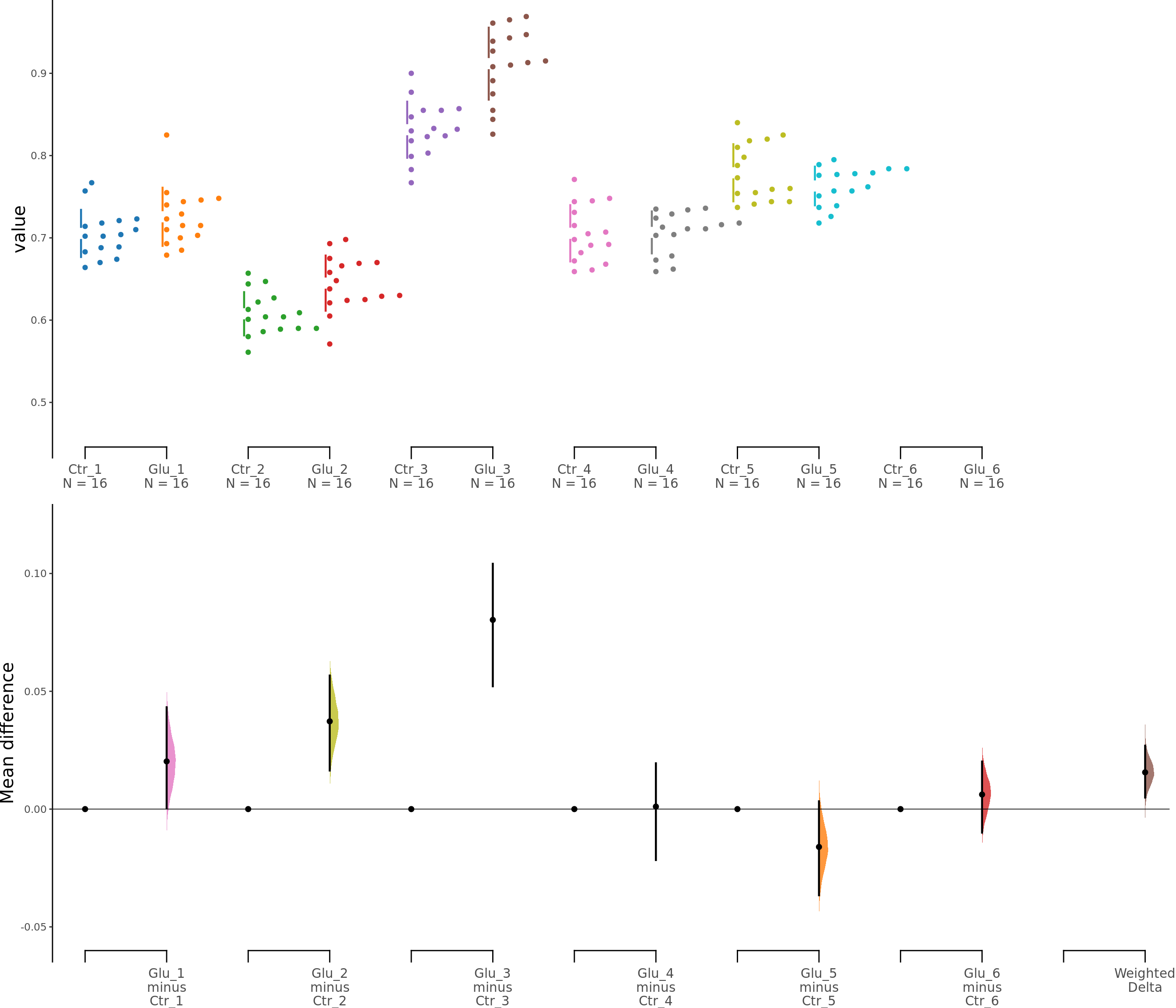
Figure 5. Effects of EPA on astrocyte viability. c. Cumming estimation plot showing astroglia viability (MTT assay) after 30 μM EPA treatment. Left panel: Colored circles represent individual data points for control (Ctr) and EPA-treated groups from 6 independent experiments. Black circles and vertical lines indicate group means with 95% confidence intervals. Right panel: Floating plots show mean differences (EPA minus Ctr) for each experiment and the overall weighted mean difference (bottom). Circles represent the point estimate of the mean difference, with vertical lines indicating 95% confidence intervals. The shaded curve represents the resampled distribution of the effect size.
100 μM of Glutamate on Astrocytes - Figure 3c
unpaired_glut <- load(df_glut,
  x = Group, y = Measurement,
  idx = list(
    c("Ctr_1", "Glu_1"),
    c("Ctr_2", "Glu_2"),
    c("Ctr_3", "Glu_3"),
    c("Ctr_4", "Glu_4"),
    c("Ctr_5", "Glu_5"),
    c("Ctr_6", "Glu_6")
  ),
  minimeta = TRUE
)print(unpaired_glut)DABESTR v2025.3.14
==================
Good afternoon!
The current time is 16:41 PM on Tuesday June 17, 2025.
ffect size(s) with 95% confidence intervals will be computed for:
1. Glu_1 minus Ctr_1
2. Glu_2 minus Ctr_2
3. Glu_3 minus Ctr_3
4. Glu_4 minus Ctr_4
5. Glu_5 minus Ctr_5
6. Glu_6 minus Ctr_6
7. weighted delta (only for mean difference)
5000 resamples will be used to generate the effect size bootstraps.unpaired_glut.mean_diff <- mean_diff(unpaired_glut)
print(unpaired_glut.mean_diff)DABESTR v2025.3.14
==================
Good afternoon!
The current time is 16:41 PM on Tuesday June 17, 2025.
The character(0) mean difference between Glu_1 and Ctr_1 is 0.02 [95%CI 0, 0.043].
The p-value of the two-sided permutation t-test is 0.0856, calculated for legacy purposes only.
The character(0) mean difference between Glu_2 and Ctr_2 is 0.037 [95%CI 0.016, 0.057].
The p-value of the two-sided permutation t-test is 0.0016, calculated for legacy purposes only.
The character(0) mean difference between Glu_3 and Ctr_3 is 0.08 [95%CI 0.052, 0.104].
The p-value of the two-sided permutation t-test is 0.0000, calculated for legacy purposes only.
The character(0) mean difference between Glu_4 and Ctr_4 is 0.001 [95%CI -0.022, 0.019].
The p-value of the two-sided permutation t-test is 0.9214, calculated for legacy purposes only.
The character(0) mean difference between Glu_5 and Ctr_5 is -0.016 [95%CI -0.037, 0.003].
The p-value of the two-sided permutation t-test is 0.1375, calculated for legacy purposes only.
The character(0) mean difference between Glu_6 and Ctr_6 is 0.006 [95%CI -0.01, 0.02].
The p-value of the two-sided permutation t-test is 0.4451, calculated for legacy purposes only.
5000 bootstrap samples were taken; the confidence interval is bias-corrected and accelerated.
Any p-value reported is the probability of observing the effect size (or greater),
assuming the null hypothesis of zero difference is true.
For each p-value, 5000 reshuffles of the control and test labels were performed.kable(unpaired_glut.mean_diff$boot_result |> select(-bootstraps))| control_group | test_group | nboots | bca_ci_low | bca_ci_high | pct_ci_low | pct_ci_high | ci | difference | weight |
|---|---|---|---|---|---|---|---|---|---|
| Ctr_1 | Glu_1 | 5000 | 0.0003849 | 0.0432387 | -0.0006859 | 0.0420594 | 95 | 0.0202500 | 965.8881 |
| Ctr_2 | Glu_2 | 5000 | 0.0163698 | 0.0566875 | 0.0168125 | 0.0568125 | 95 | 0.0372500 | 1102.0093 |
| Ctr_3 | Glu_3 | 5000 | 0.0521250 | 0.1041250 | 0.0531891 | 0.1056234 | 95 | 0.0803125 | 649.9001 |
| Ctr_4 | Glu_4 | 5000 | -0.0216248 | 0.0194375 | -0.0196875 | 0.0210000 | 95 | 0.0010625 | 1098.9137 |
| Ctr_5 | Glu_5 | 5000 | -0.0365625 | 0.0033125 | -0.0359359 | 0.0039984 | 95 | -0.0160625 | 1136.8508 |
| Ctr_6 | Glu_6 | 5000 | -0.0099801 | 0.0201875 | -0.0090625 | 0.0207500 | 95 | 0.0061875 | 1960.9205 |
| Minimeta Overall Test | Minimeta Overall Test | 5000 | 0.0049018 | 0.0269089 | 0.0154685 | 0.0157784 | 95 | 0.0155969 | 1.0000 |
dabest_plot(unpaired_glut.mean_diff)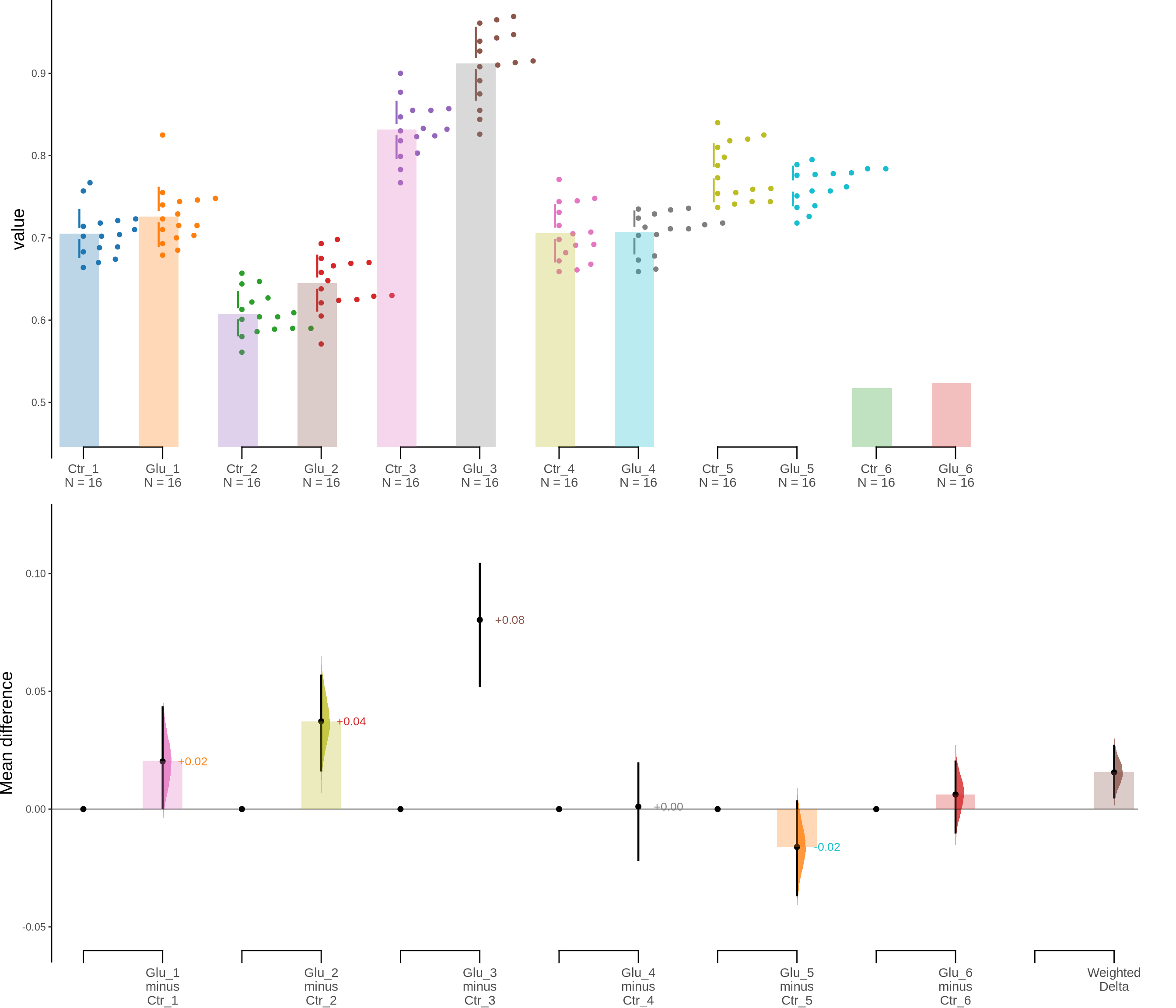
| Version | Author | Date |
|---|---|---|
| cccdace | EugOT | 2025-06-17 |
Figure 3. Effects of glutamate on astrocyte viability. c. Cumming estimation plot showing astroglia viability (MTT assay) after 100 μM glutamate treatment. Left panel: Colored circles represent individual data points for control (Ctr) and glutamate-treated (Glu) groups from 6 independent experiments. Black circles and vertical lines indicate group means with 95% confidence intervals. Right panel: Floating plots show mean differences (Glu minus Ctr) for each experiment and the overall weighted mean difference (bottom). Circles represent the point estimate of the mean difference, with vertical lines indicating 95% confidence intervals. The shaded curve represents the resampled distribution of the effect size.
sessionInfo()R version 4.3.3 (2024-02-29)
Platform: x86_64-conda-linux-gnu (64-bit)
Running under: Ubuntu 24.04.2 LTS
Matrix products: default
BLAS/LAPACK: /data/Cinquina_2024/.pixi/envs/default/lib/libopenblasp-r0.3.29.so; LAPACK version 3.12.0
locale:
[1] LC_CTYPE=en_US.UTF-8 LC_NUMERIC=C
[3] LC_TIME=en_US.UTF-8 LC_COLLATE=en_US.UTF-8
[5] LC_MONETARY=en_US.UTF-8 LC_MESSAGES=en_US.UTF-8
[7] LC_PAPER=en_US.UTF-8 LC_NAME=C
[9] LC_ADDRESS=C LC_TELEPHONE=C
[11] LC_MEASUREMENT=en_US.UTF-8 LC_IDENTIFICATION=C
time zone: Europe/Vienna
tzcode source: system (glibc)
attached base packages:
[1] stats graphics grDevices utils datasets methods base
other attached packages:
[1] skimr_2.1.5 magrittr_2.0.3 lubridate_1.9.4 forcats_1.0.0
[5] stringr_1.5.1 dplyr_1.1.4 purrr_1.0.4 readr_2.1.5
[9] tidyr_1.3.1 tibble_3.3.0 ggplot2_3.5.2 tidyverse_2.0.0
[13] dabestr_2025.3.14 RColorBrewer_1.1-3 knitr_1.50 here_1.0.1
[17] workflowr_1.7.1
loaded via a namespace (and not attached):
[1] beeswarm_0.4.0 gtable_0.3.6 xfun_0.52 bslib_0.9.0
[5] processx_3.8.6 callr_3.7.6 tzdb_0.5.0 vctrs_0.6.5
[9] tools_4.3.3 ps_1.9.1 generics_0.1.4 parallel_4.3.3
[13] pkgconfig_2.0.3 lifecycle_1.0.4 compiler_4.3.3 farver_2.1.2
[17] git2r_0.35.0 ggsci_3.2.0 repr_1.1.7 getPass_0.2-4
[21] vipor_0.4.7 httpuv_1.6.15 htmltools_0.5.8.1 sass_0.4.10
[25] yaml_2.3.10 later_1.4.2 pillar_1.10.2 crayon_1.5.3
[29] jquerylib_0.1.4 whisker_0.4.1 ggmin_0.0.0.9000 cachem_1.1.0
[33] boot_1.3-31 tidyselect_1.2.1 digest_0.6.37 stringi_1.8.7
[37] labeling_0.4.3 cowplot_1.1.3 rprojroot_2.0.4 fastmap_1.2.0
[41] grid_4.3.3 cli_3.6.5 base64enc_0.1-3 effsize_0.8.1
[45] withr_3.0.2 scales_1.4.0 promises_1.3.3 bit64_4.6.0-1
[49] ggbeeswarm_0.7.2 timechange_0.3.0 rmarkdown_2.29 httr_1.4.7
[53] bit_4.6.0 hms_1.1.3 evaluate_1.0.3 rlang_1.1.6
[57] Rcpp_1.0.14 glue_1.8.0 rstudioapi_0.17.1 vroom_1.6.5
[61] jsonlite_2.0.0 R6_2.6.1 fs_1.6.6